For a start, we will need some data. Instead of generating it in gnuplot, I will just post my data file, which reads as follows
1 2 3 1 2 5
2 2 4 2 3 1
3 4 3 6 1 1
4 2 3 1 1 4
5 3 2 5 4 3
6 2 3 6 5 3
We have six columns here, but only five are the data: the first columns is for indexing, or whatever you like. This does not change the idea. In what follows, I will call this file '3fill.dat'
Now, our first script looks like this
reset
unset key
unset colorbox
set ytics offset 0,-1
set ticslevel 0
min = 0
col = 5
DATA = ""
DATA2 = ""
PALETTE = "set palette defined ("
pr(x, y) = sprintf("%f %f\n", x, y)
zero_line(x, y) = DATA.sprintf("\n").DATA2.sprintf("\n%f %f\n", x, y)
zero_pal(x) = sprintf("%d %.3f %.3f %.3f", x, rand(0), rand(0), rand(0))
f(x, y) = ($0 == 0 ? (DATA = zero_line($1, x), DATA2 = pr($1, min), PALETTE = PALETTE.zero_pal(y).", ") : \
(DATA = DATA.pr($1, x), DATA2 = DATA2.pr($1, min)), x)
plot for [i=2:col+1] '3fill.dat' u 1:(f(column(i), i))
DATA = DATA.sprintf("\n").DATA2
set print '3fill.tab'
print DATA
set print
eval(PALETTE.zero_pal(col+2).")")
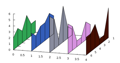
splot for [i=0:col-1] '3fill.tab' every :::(2*i)::(2*i+1) u 1:(i):2:(i+2) w pm3d
and the figure produced is here
Once you absorb it, the script is really simple. The first line where something actually happens is where we define DATA, DATA2, and PALETTE. What we will do is to read in the data from the file, and then add the numbers to a string. Once we have read all data, we print the string to a file, and then use that file as our new data file. The reason for this is that we have, in some sense, for to duplicate our data: in each column, we have one set of data, and what this set determines is a curve. In order to produce a fence, however, we need a surface. The simples way of getting this surface is to print the data twice. Of course, we have to modify the data a bit, but this is the only trick here.
We define three functions, pr, which is just a short-hand for formatted printing of two numbers, zero_line, which is again, a printing routine, when the record number is zero, i.e., when we are processing the first data point in each column, and zero_pal, which generates a new palette colour, as we enter a new column. If you are satisfied with some readily available palette, you can skip this function, and any calls to it.
Next, we define a function, f(x,y), which makes use of the three above-mentioned functions, and amounts to the data-duplication process. In order to reduce the complexity of the problem, we will print each column, and its duplicate in the same file. This, however, means that we have got to differentiate between various data sets. We do this by inserting and extra blank line each time we are faced with a new column. This is why we have to distinguish the $0 == 0 case in f(x,y). Also, the palette has to be re-defined only if there is a new data set.
If you watch carefully here, there are two strings, DATA, and DATA2. DATA2 is to hold the duplicate, while DATA is an ever-expanding string with the original, and the duplicate data. In the duplicate, we don't actually hold any duplicate, we simply print the indices (these are in the first column), and a constant number, min, which we defined at the very beginning. The value of this determines how tall (or how deep) the fences will be.
In order to generate the duplicated data set, first we call a dummy plot with f(x,y), add the last duplicate, DATA2 to DATA (this is required, because we concatenate DATA and DATA2 only, when $0 == 0, i.e., the last data set is not added to DATA automatically. Having defined DATA, we print the everything to a file. Note that we could process a number of columns easily, thanks to the for loop in the dummy plot.
At this point, we have everything in the new data file, we have only got to plot it. Recall, that all columns are in one file now, and we have to separate them in the new plot. This is why we use the 'every' keyword when stepping through the data sets.
We can easily add a grid to the figure, if we call another plot at the very end of our script: just add
for [i=0:col-1] '3fill.tab' every :::(2*i)::(2*i+1) u 1:(i):2 w l lt -1
after the last line, and get the following figure
If the order of the plots is exchanged, the "wires" will be covered by the panes of the fence, so it will not give this impression of semi-transparency. This is it for today. In my next post, I will elaborate on for what else we can use the trick above.
Cheers,
Zoltán